Writing this one took forever. From trying to understand the architecture on my whiteboard to asking a language model to create a 3D end-to-end working model for me to capture the nuances.
Got this idea from a couple of places: first it was the Welch Labs video on MLA, then saurabh's blog on writing Llama3 in 100 lines of pure JAX as well as Alessio's blog: Vision Transformer in pure JAX
I assume if you're reading this one then you are familiar with python and understand the basics of transformer architectures. If not then no worries i'll try my best to be as lucid as i can be. Also, and of course, this won't be a complete 671B parameter implementation of the V3 architecture but merely a 36.2M params implementation owing to the fact that i am GPU poor.
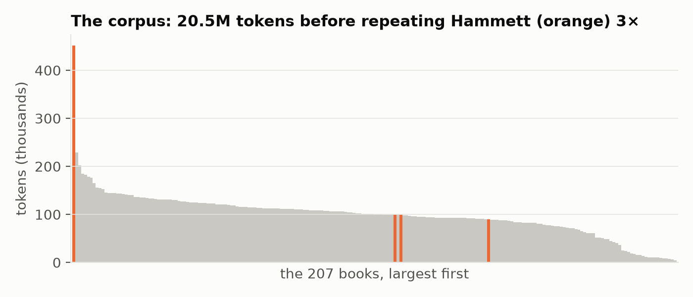
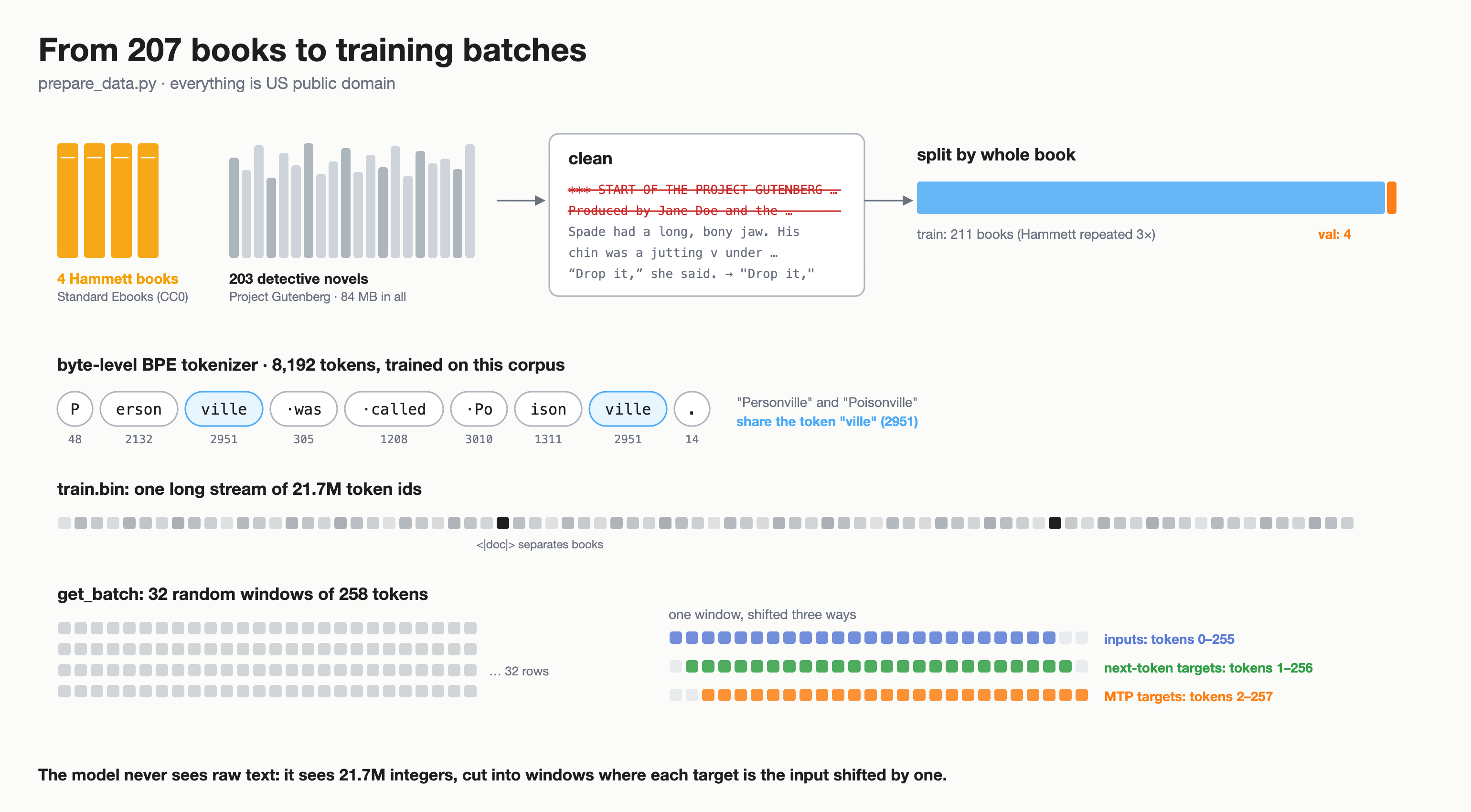
Couple of things before we dive in: I have trained the model on a MacBook Air M5 (24GB, 10-core GPU) through Apple's jax-metal plugin, which plugs Apple's GPU into JAX as a PJRT, more on this later. And secondly, i saw that at a lot of places the shakespeare dataset is used so I wanted it to be different just for the sake of it and used various books by Hammett, and numerous books from the Project Gutenberg comprising of Sherlock Holmes, Edgar Wallace, Father Brown, Anna Katharine, etc. You can build the dataset with prepare_data.py in the repo. Initially I thought of using a dataset of film scripts, but getting those legally was a bummer so i went ahead with these. Also, i used Claude Opus 5.5 to draw some of the images that are explaining the architecture.
High level overview of the Architecture
The basic skeleton of the architecture at its root is a decoder only model. You send in tokens -> they get vectorized and each token is looked up in the embedding table -> this vector will be the residual stream, every layer will read from it and add back to it. This would happen through N blocks and each block will do the same 2 steps -> Attention + FFN -> both steps would read a normalized copy of the residual stream and add their output back. And then finally the o/p head would turn the vector into a score for every word in the vocabulary.
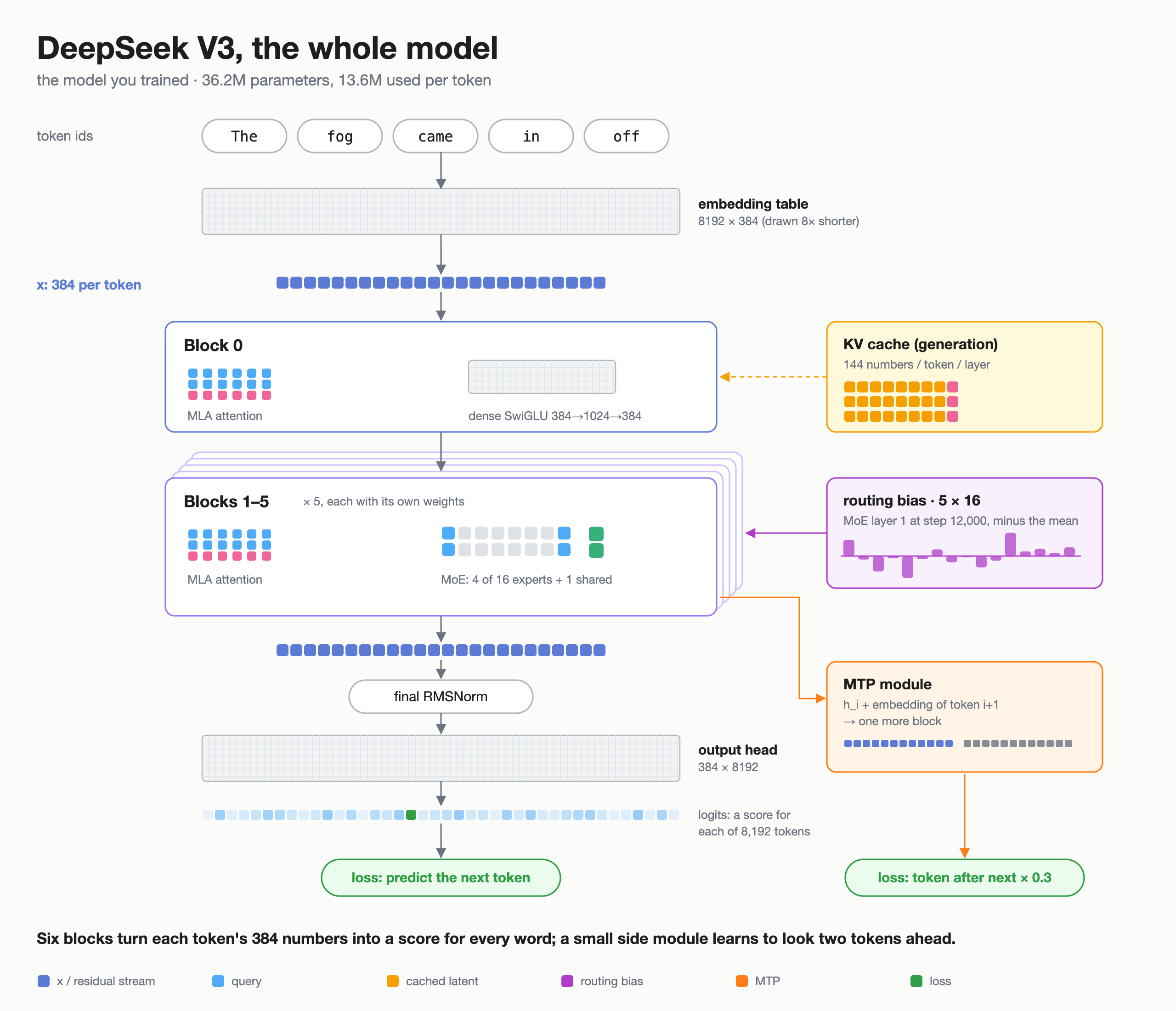
Now comes the idea that makes you finally think, the places where V3 showed novelty.
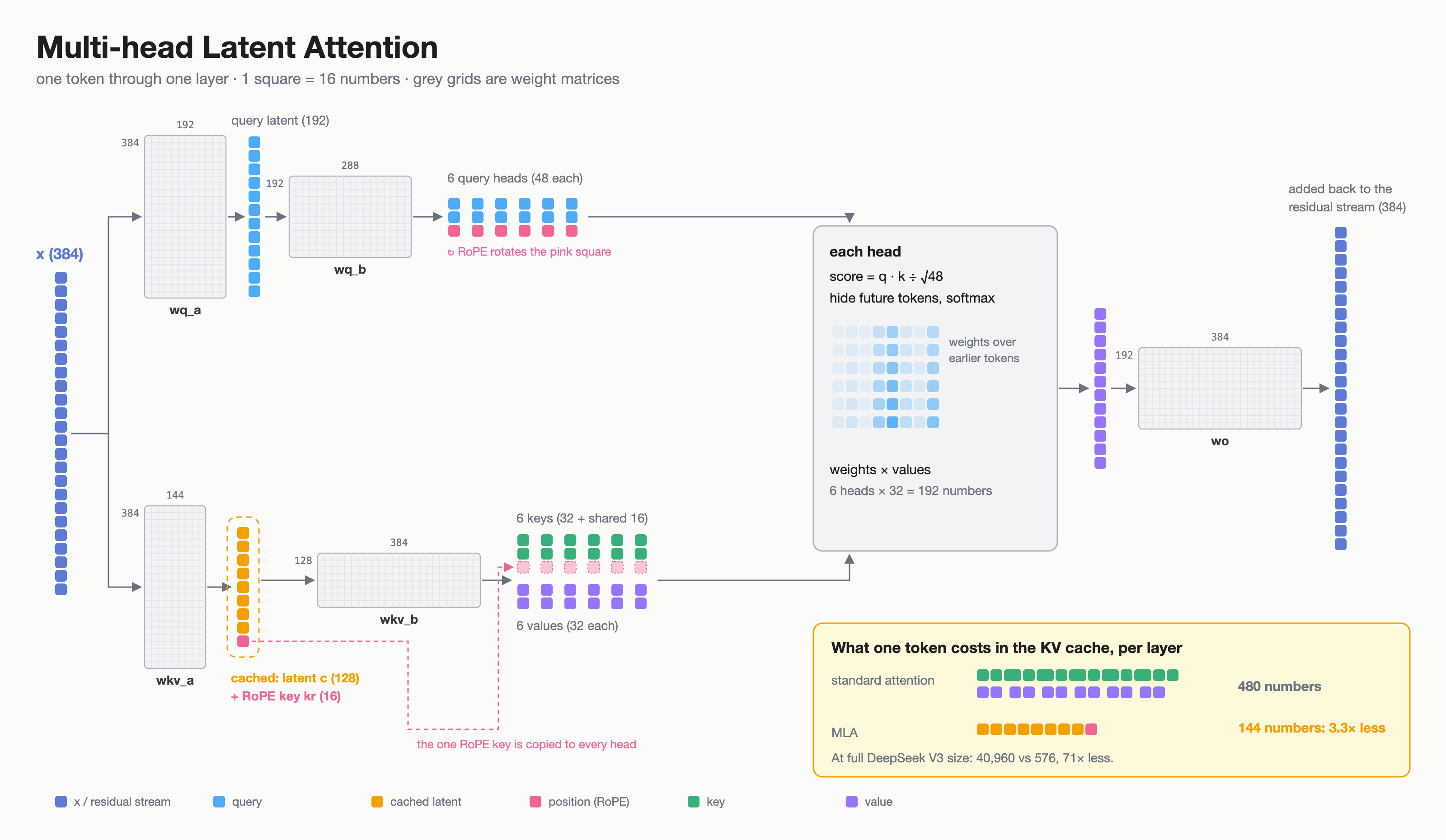
1) Multi-head Latent Attention - I would highly encourage y'all to go through the Welch Labs video for this cause that is GOATED. So while generating a model caches every past token's keys and values (KV cache) and by basic logic, at long contexts that cache eats a lot of memory (yes the one which sam altman said should belong in the datacenters and not with individuals lol). What MLA does is that it compresses each token into one small latent vector and caches only that. The KV for every head are rebuilt from it whenever needed.
2) DeepSeekMOE - That is kind of self explanatory, that one big FFN becomes many small FFNs. A router just scores every expert for each token and sends tokens to the top k. That's why its mentioned that original V3 has 671B parameters but only uses 37B parameters per token.
3) Aux-loss-free balancing - See there's a nuance here as well. If we would keep the router idle for sometime, then it gets lazy in properly routing and gives few experts more tokens and then they get better and rest go by unused. So V3 just becomes a damn Robin Hood and overused experts gets their bias nudged down after every step and underused ones gets an up.
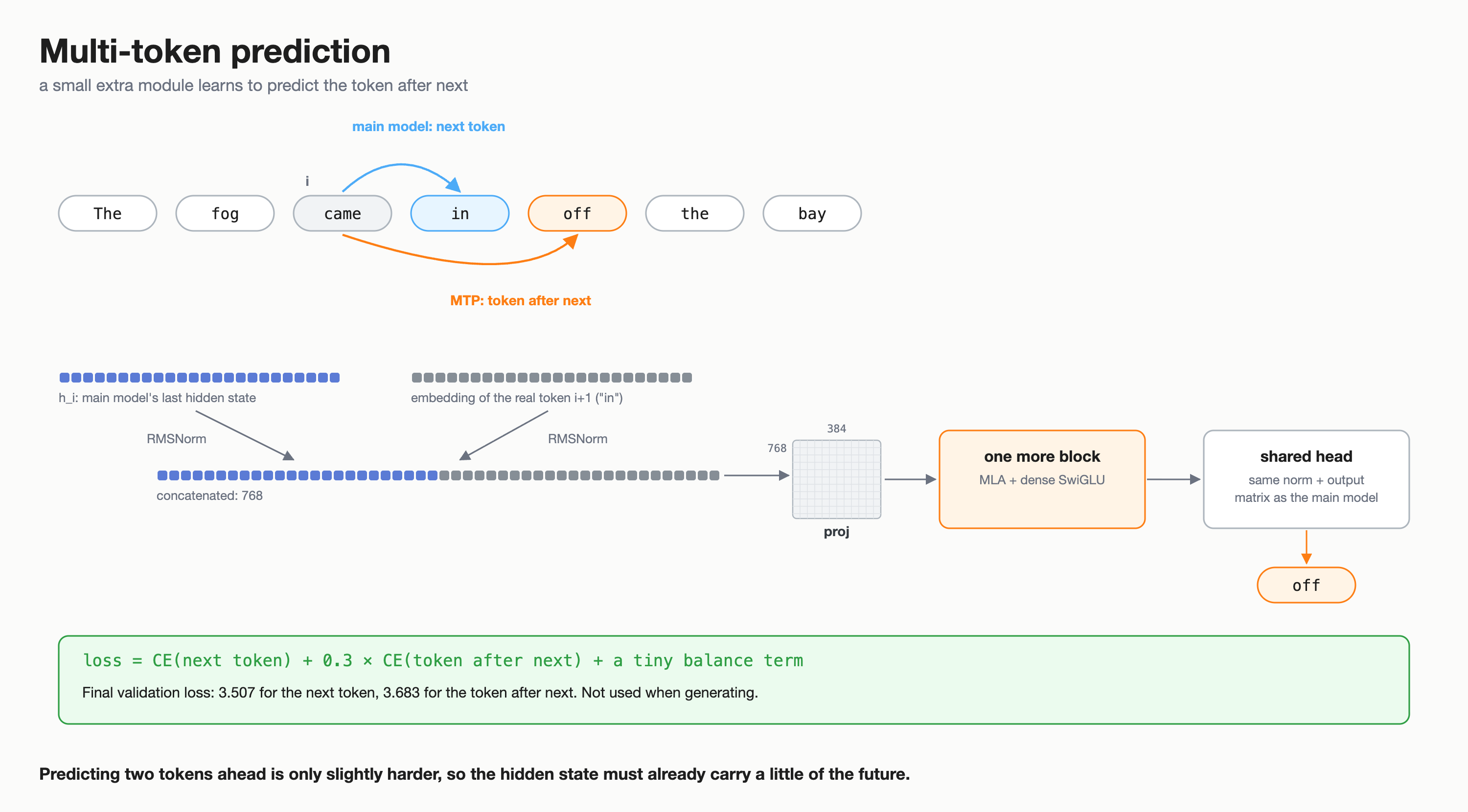
4) Multi Token Prediction - So generally we just see the next token but here we predict the token after the next one as well to give the model a push to plan a little ahead.
The other differences such that the original model is 671B/37B and my implementation is 36.2M/13.6M and og model had 7168 dims whereas we have 384 dims and etc. will be covered along with the implementation itself. You can go through the Deepseek V3 technical report if you want to go in-depth.
Now let's get started
Now why i liked (felt cool) using JAX? it looks like numpy but doesn't run line by line. When you wrap a function in jax.jit, it compiles it in place. jit: just in time. Also JAX doesn't really care if the program runs on GPU or TPU or CPU, it only needs a backend that can compile and run XLA programs for that chip.
An “XLA program” is your Python function rewritten as a plain list of array operations, with all the Python stripped out.
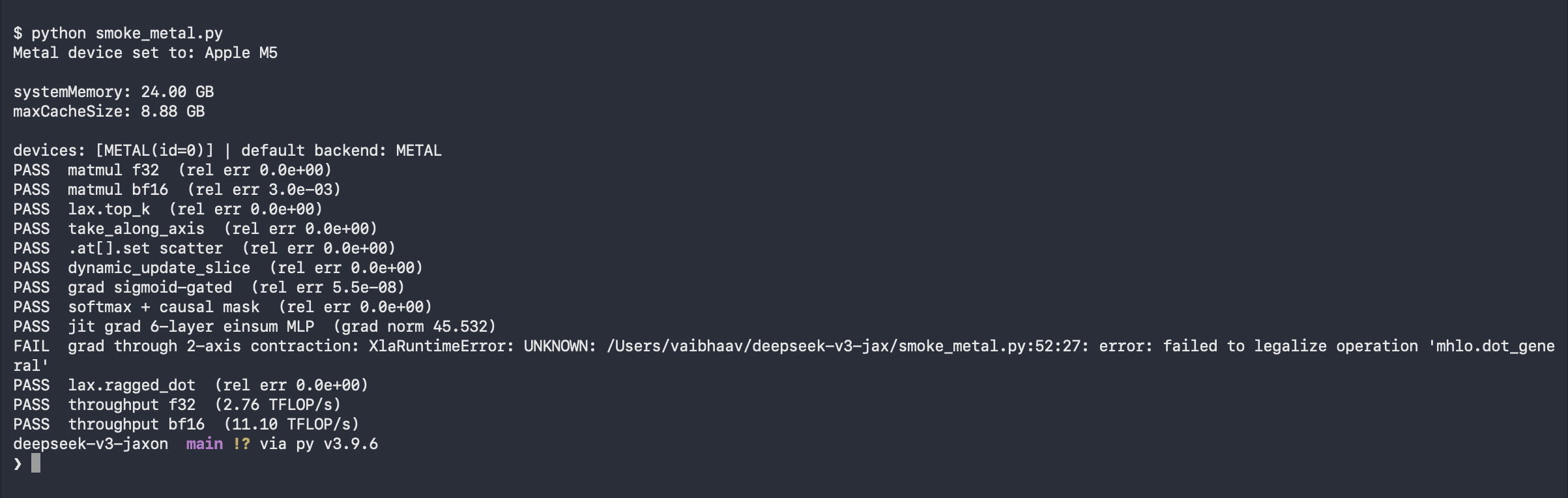
The model runs on a mac GPU as i mentioned earlier, all thanks to Apple's jax-metal plugin, a PJRT plugin. It translates XLA programs into Metal which is Apple's GPU API and runs them on Mac's GPU. The catch is that it only works with jax==0.4.34 cause Apple hasn't updated jax-metal in a while so newer JAX breaks it.
uv venv -p 3.12 .venv
uv pip install --python .venv/bin/python -r requirements.txt
.venv/bin/python smoke_metal.py
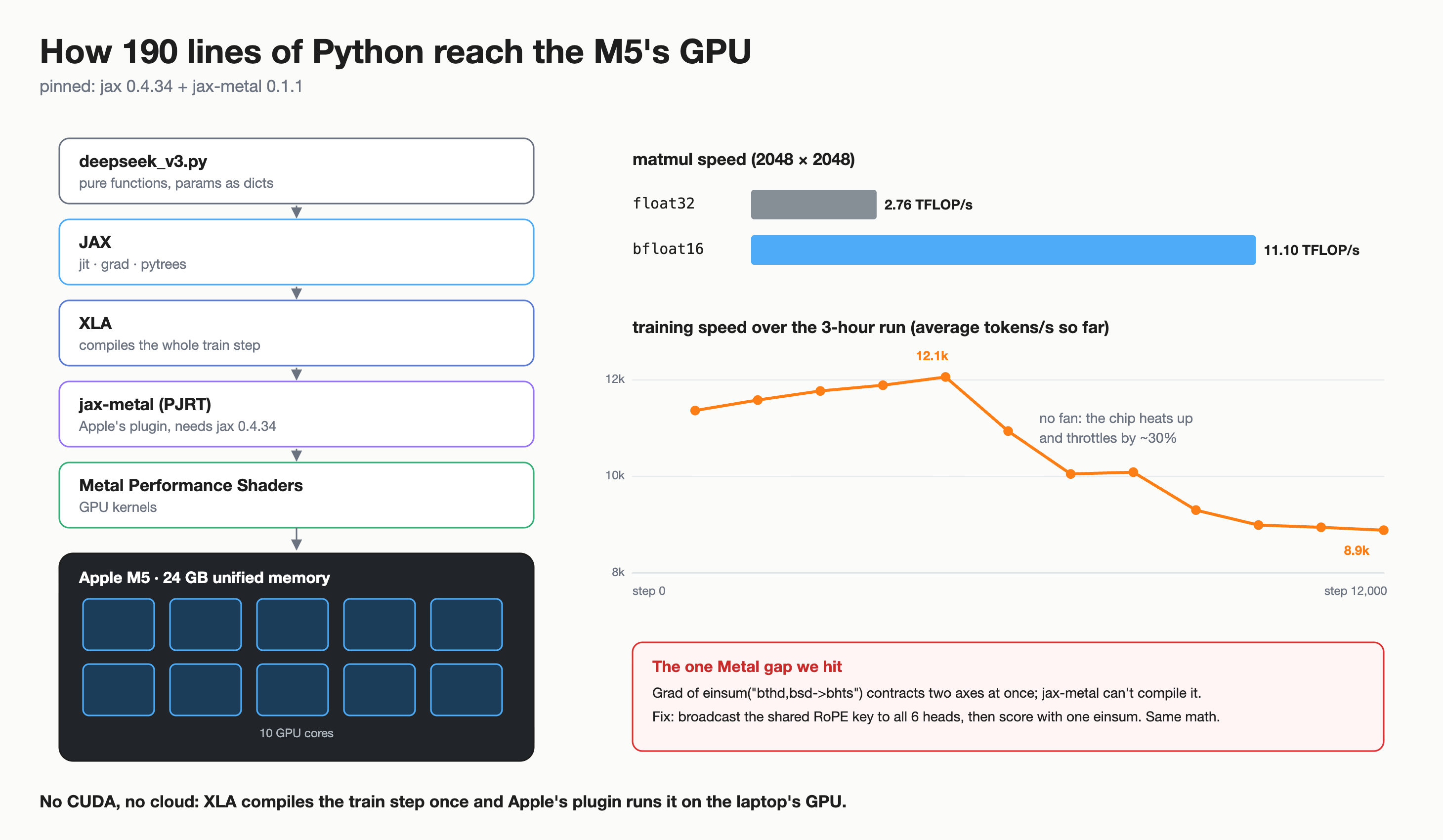
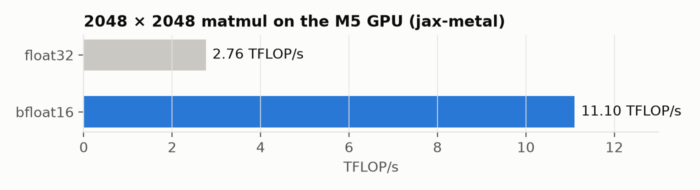
Also bf16 matmuls run ~4x faster than f32 here which i will discuss more in training
The config
I mentioned earlier that the real V3 has 671B/37B parameters whereas this one has 36.2M/13.6M. Other contrasts include that; OG had 61 layers (3+58) and ours has 6 layers (1+5); OG had 128 heads and mine has 6; you know what? i should add a comparative table instead.
| DeepSeek V3 | Ours | |
|---|---|---|
| params (total / active per token) | 671B / 37B | 36.2M / 13.6M |
| layers (dense + MoE) | 61 (3 + 58) | 6 (1 + 5) |
| d_model | 7168 | 384 |
| attention heads | 128 | 6 |
| MLA query / KV latent rank | 1536 / 512 | 192 / 128 |
| per-head dims (nope / rope / v) | 128 / 64 / 128 | 32 / 16 / 32 |
| experts | 1 shared + 256 routed, top-8 | 1 shared + 16 routed, top-4 |
| expert hidden size | 2048 | 256 |
| vocab | ~129K | 8192 |
| context | 4K (extended to 128K) | 256 |
overall my model is 1/18500th of V3 if you wanna look it from that perspective
from dataclasses import dataclass
import jax, jax.numpy as jnp
import optax


@dataclass(frozen=True)
class Config:
    vocab: int = 8192
    d_model: int = 384
    n_layers: int = 6
    n_dense: int = 1           # first layers use a dense FFN instead of MoE
    n_heads: int = 6
    q_rank: int = 192          # MLA: low-rank query compression
    kv_rank: int = 128         # MLA: low-rank joint key/value compression (this is what gets cached)
    d_nope: int = 32           # per-head query/key dims without RoPE
    d_rope: int = 16           # per-head query/key dims with RoPE (key part shared across heads)
    d_v: int = 32              # per-head value dim
    d_ff: int = 1024           # dense FFN hidden size
    n_shared: int = 1          # MoE: always-on shared experts
    n_routed: int = 16         # MoE: routed experts
    top_k: int = 4             # MoE: routed experts per token
    d_expert: int = 256        # MoE: hidden size of each expert
    route_scale: float = 1.0   # MoE: scale on the normalized gate weights
    gamma: float = 1e-3        # bias update speed for aux-loss-free balancing
    alpha_seq: float = 1e-4    # weight of the complementary sequence-wise balance loss
    n_mtp: int = 1             # multi-token prediction depth
    mtp_lambda: float = 0.3    # weight of the MTP loss
    seq_len: int = 256
    batch: int = 32
    rope_theta: float = 10000.0
    init_std: float = 0.02
    dtype: str = "bfloat16"    # compute dtype; weights and optimizer state stay float32


SMALL = Config(n_layers=4, n_routed=8, top_k=2, seq_len=128, batch=16)
TINY = Config(vocab=64, d_model=32, n_layers=2, n_heads=2, q_rank=16, kv_rank=8, d_nope=8, d_rope=4, d_v=8,
              d_ff=64, n_routed=4, top_k=2, d_expert=16, seq_len=16, batch=2, dtype="float32")   # tests
Initializing the weights
so pure JAX has no nn.Module or layer classes and all the model's weights are one nested dict of arrays. This is already pointed out in Saurabh's and Alessio's blog.
Couple of things that i would like to point out: there's no global seed in JAX, instead you pass a key and jax.random.split for every weight. Secondly we stack each expert weight across all 16 experts into a single 3D block - [16, 384, 256] - so the GPU can work through all of them in a single call. Also the routed experts hold about 23.6M of the 36.2M parameters which is about 2/3 of the model and most of it sits idle for any given token.
def normal(key, shape, std):
    return jax.random.normal(key, shape) * std


def init_swiglu(cfg, key, hidden):
    k1, k2, k3 = jax.random.split(key, 3)
    d, s = cfg.d_model, cfg.init_std
    return {"w1": normal(k1, (d, hidden), s), "w3": normal(k2, (d, hidden), s), "w2": normal(k3, (hidden, d), s)}


def init_mla(cfg, key):
    k = jax.random.split(key, 5)
    d, H, s = cfg.d_model, cfg.n_heads, cfg.init_std
    return {"wq_a": normal(k[0], (d, cfg.q_rank), s), "q_norm": jnp.ones(cfg.q_rank),
            "wq_b": normal(k[1], (cfg.q_rank, H * (cfg.d_nope + cfg.d_rope)), s),
            "wkv_a": normal(k[2], (d, cfg.kv_rank + cfg.d_rope), s), "kv_norm": jnp.ones(cfg.kv_rank),
            "wkv_b": normal(k[3], (cfg.kv_rank, H * (cfg.d_nope + cfg.d_v)), s),
            "wo": normal(k[4], (H * cfg.d_v, d), s)}


def init_moe(cfg, key):
    k = jax.random.split(key, 5)
    d, E, h, s = cfg.d_model, cfg.n_routed, cfg.d_expert, cfg.init_std
    return {"router": normal(k[0], (d, E), s), "shared": init_swiglu(cfg, k[1], cfg.n_shared * h),
            "experts": {"w1": normal(k[2], (E, d, h), s), "w3": normal(k[3], (E, d, h), s),
                        "w2": normal(k[4], (E, h, d), s)}}


def init_block(cfg, key, moe):
    k1, k2 = jax.random.split(key)
    ffn = {"moe": init_moe(cfg, k2)} if moe else {"ffn": init_swiglu(cfg, k2, cfg.d_ff)}
    return {"norm_attn": jnp.ones(cfg.d_model), "attn": init_mla(cfg, k1), "norm_ffn": jnp.ones(cfg.d_model), **ffn}


def init_params(cfg, key):
    ke, kh, kl, km = jax.random.split(key, 4)
    d = cfg.d_model
    layers = [init_block(cfg, k, moe=i >= cfg.n_dense) for i, k in enumerate(jax.random.split(kl, cfg.n_layers))]
    mtp = [{"norm_h": jnp.ones(d), "norm_e": jnp.ones(d), "proj": normal(k1, (2 * d, d), cfg.init_std),
            "block": init_block(cfg, k2, moe=False)}
           for k1, k2 in (jax.random.split(k) for k in jax.random.split(km, cfg.n_mtp))]
    return {"embed": normal(ke, (cfg.vocab, d), cfg.init_std), "head": normal(kh, (d, cfg.vocab), cfg.init_std),
            "norm_f": jnp.ones(d), "layers": layers, "mtp": mtp}


def n_params(params):
    return sum(x.size for x in jax.tree.leaves(params))
Tokenization + BPE
I hope we already know the need for tokenization if you've made it this far in the blog. The model only sees numbers so text needs to become ids first, but we can't give 1 id per character cause then the sequences will be very long. We also can't give 1 id per word, even though that would make the sequences shorter, cause the vocabulary has way too many words to have an id of their own + on words which will be unseen, the model would likely give <unknown>. That's why we use byte pair encoding, where common words get a single id + the rare words get broken down into smaller chunks. For e.g, according to the dataset i am using, fog, Holmes, cigarette (along with the space before them), get a single id whereas unbelievably gets broken down into un | b | elie | v | ably.
tok = Tokenizer(models.BPE())
tok.pre_tokenizer = pre_tokenizers.ByteLevel(add_prefix_space=False)
tok.decoder = decoders.ByteLevel()
tok.train_from_iterator(train, trainers.BpeTrainer(vocab_size=VOCAB, special_tokens=[DOC],
                                                   initial_alphabet=pre_tokenizers.ByteLevel.alphabet()))
tok.save(str(DATA / "tokenizer.json"))

for name, docs in [("train", train), ("val", val)]:
    ids = [[0] + e.ids for e in tok.encode_batch(docs)]
    arr = np.concatenate(ids).astype(np.uint16)
    assert arr.max() < 65536 and tok.token_to_id(DOC) == 0
    arr.tofile(DATA / f"{name}.bin")
Embedding and residual stream
We now know that the model has a number assigned for the words, but just a number can't tell you anything about the actual word so we keep a table of 8192 rows, one per token and each row has a list of 384 numbers. What we're doing here is creating a lookup table. All those numbers are the word's description and they start out randomly but the training slowly tunes them so that similar words would end up with similar numbers.
Now these 384 numbers are carried by the token through the model, and as i have told above we have 6 blocks performing Attention and FFN.
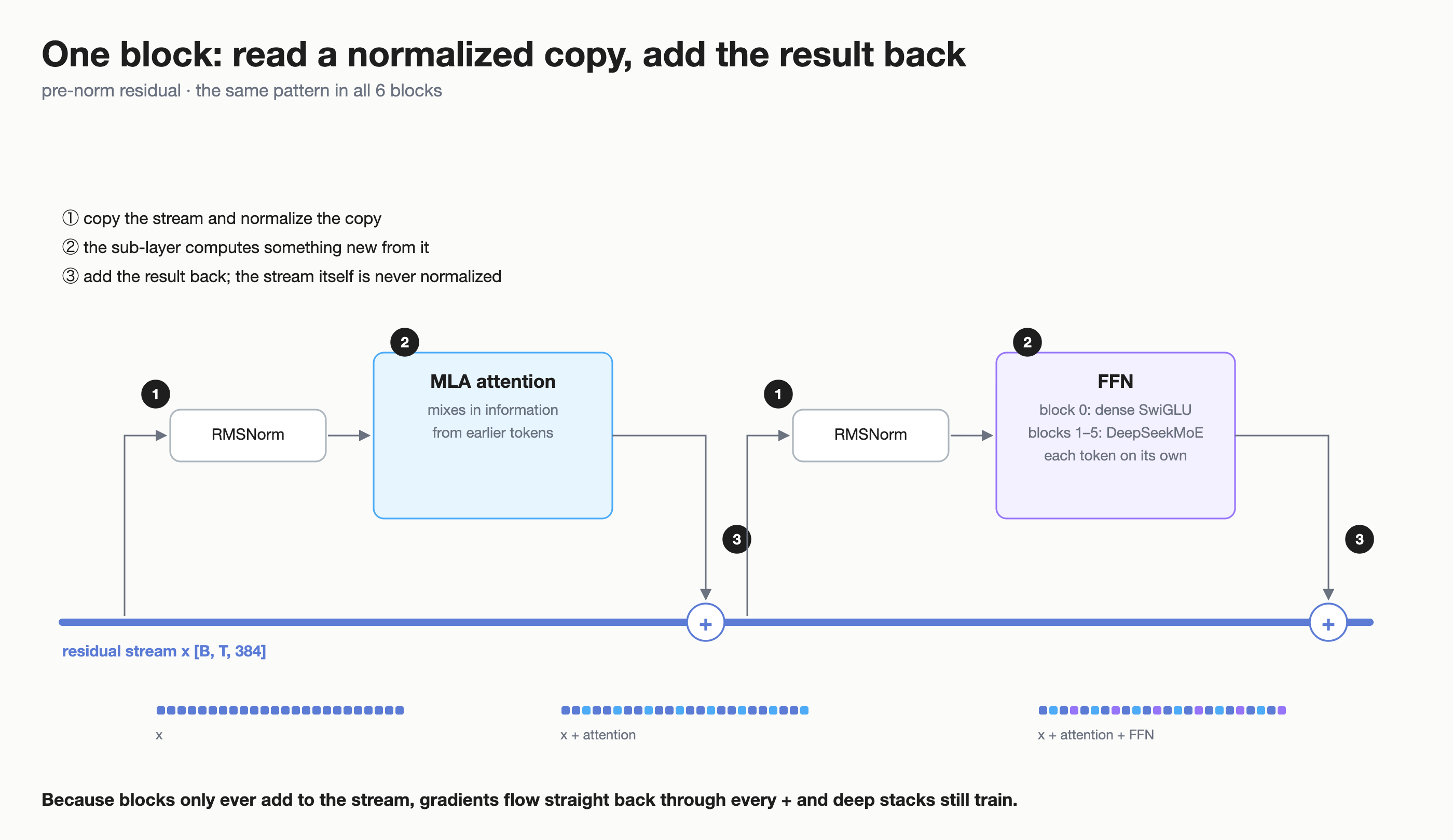
In the Attention layer - x is RMS normalized then each token looks back at the tokens before it -> then decides which ones matter the most and pulls the info from them. the resultant vector is a vector of the same size as x and that gets added to x
whereas in the FFN - the updated x is normalized again and passed through a SwiGLU FFN (in layers 1–5 this FFN is swapped for MoE, more on that later) -> the FFN works on each position seperately so that there's no mixing across tokens and the output f is added to x again: x = x + f
def block(p, bias, x, cos, sin, cfg, cache=None, pos=0):
    a, cache = mla(p["attn"], rms_norm(x, p["norm_attn"]), cos, sin, cfg, cache, pos)
    x = x + a
    h = rms_norm(x, p["norm_ffn"])
    f, aux = moe(p["moe"], bias, h, cfg) if "moe" in p else (swiglu(p["ffn"], h), None)
    return x + f, aux, cache


def forward(params, biases, tokens, cfg, caches=None, pos=0):
    cos, sin = rope(cfg, pos + jnp.arange(tokens.shape[1]))
    x, auxes, new_caches = params["embed"][tokens], [], []                # [B,T,d]
    for i, p in enumerate(params["layers"]):
        bias = biases[i - cfg.n_dense] if i >= cfg.n_dense else None     # one bias vector per MoE layer
        x, aux, c = block(p, bias, x, cos, sin, cfg, None if caches is None else caches[i], pos)
        new_caches.append(c)
        if aux is not None: auxes.append(aux)
    logits = rms_norm(x, params["norm_f"]) @ params["head"]               # [B,T,V]
    aux = {"load": jnp.stack([a["load"] for a in auxes]), "seq_loss": sum(a["seq_loss"] for a in auxes)}
    return logits, x, aux, new_caches
RMS Norm
The numbers moving through the token can grow huge or can go really tiny, and ofcourse that would affect output. So right before the token passes through the attention and FFN layer it passes through root mean square normalization where it rescales it to a standard size.
def rms_norm(x, w, eps=1e-6):
    return x * jax.lax.rsqrt(jnp.mean(x * x, -1, keepdims=True) + eps) * w
RoPE
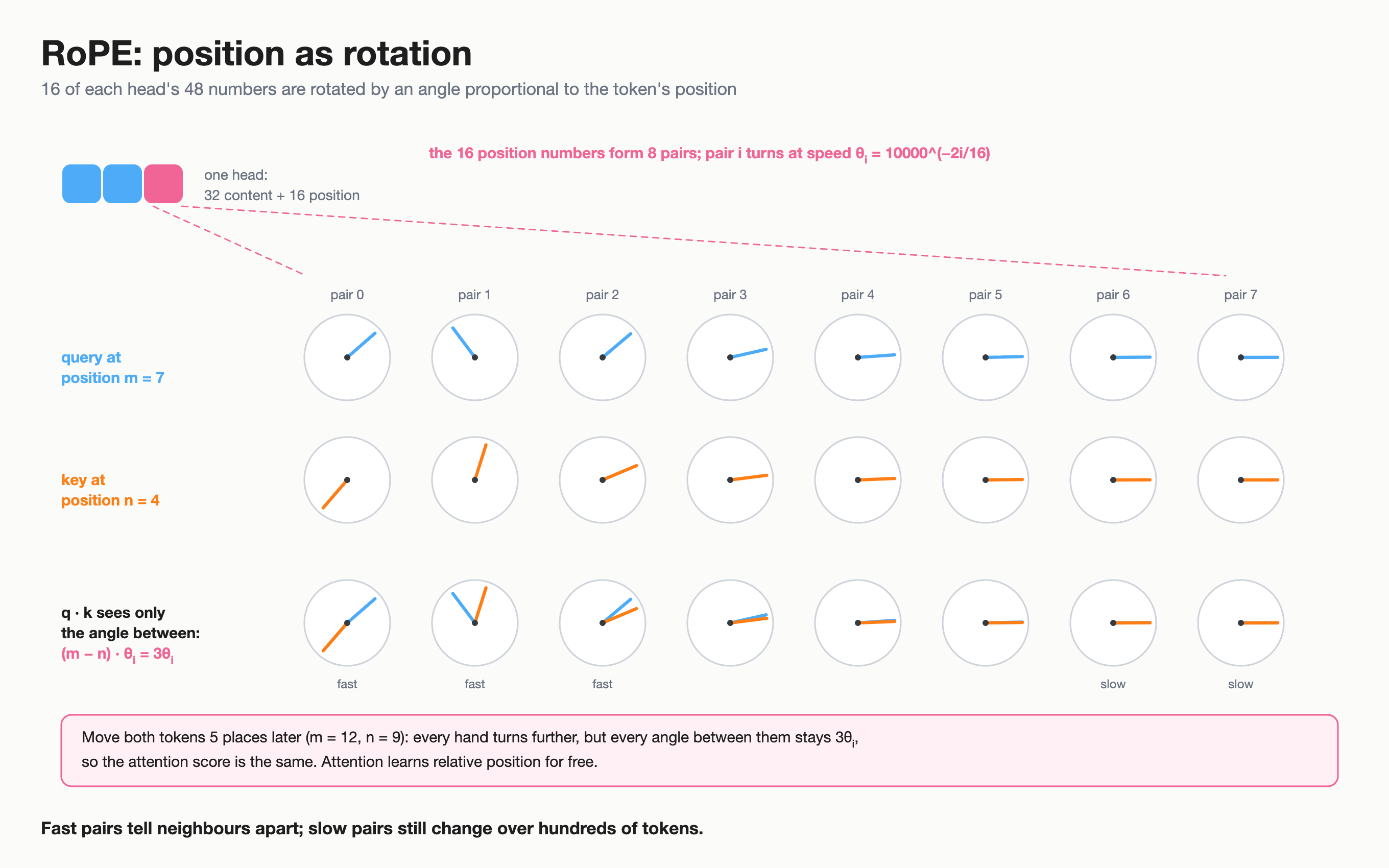
We know that attention compares tokens by multiplying their vectors but that dot product doesn't know where each token really is, in the sentence. Rotary Positional Embeddings fixes this issue by rotating the vector by an angle that depends on its position. So for e.g. there's fog and came are 1 apart in terms of position, then they would look the same whether they are at 4 and 5 or 101 and 102 i.e. when you would compare two vectors the result depends only on how far apart they are. The difference in V3 is that it rotates only 16 of each head's Q/K dims and the other 32 gets no rotation and the rotated key part is one vector shared by all 6 heads.
def rope(cfg, positions):
    freqs = cfg.rope_theta ** -(jnp.arange(0, cfg.d_rope, 2) / cfg.d_rope)    # [d_rope/2]
    angles = positions[:, None] * freqs[None, :]                               # [T, d_rope/2]
    return jnp.cos(angles), jnp.sin(angles)


def apply_rope(x, cos, sin):
    cos, sin = (a.reshape(a.shape[0], *[1] * (x.ndim - 3), a.shape[1]) for a in (cos, sin))
    x1, x2 = jnp.split(x, 2, axis=-1)
    return jnp.concatenate([x1 * cos - x2 * sin, x1 * sin + x2 * cos], -1)
DeepSeek's novelty
Multi-head Latent Attention
This is where we get into V3's waters. You must have seen how the usual Attention architecture goes by. Every token makes a query, key and value for every head, and that is goated and was working perfectly fine. The issue was that while generating them they cache every past token's K and V for every head and every layer -> and this will be really painful when you will increase the context window.
What V3 does differently is that it caches just a small summary c of each token instead of complete K and V and then rebuild KV from that whenever needed. And that is the reason RoPE can't rotate all the keys cause it can't rotate a summary.
Cache per token per layer: 480 → 144 numbers here, 40,960 → 576 in the real V3. At a 128K context over 61 layers in bf16, that's ~655 GB vs ~9 GB.
def init_cache(cfg, B, n_layers):
    # MLA caches only the compressed latent c and the shared RoPE key, not per-head K and V
    return [{"c": jnp.zeros((B, cfg.seq_len, cfg.kv_rank)), "kr": jnp.zeros((B, cfg.seq_len, cfg.d_rope))}
            for _ in range(n_layers)]


def mla(p, x, cos, sin, cfg, cache=None, pos=0):
    B, T, _ = x.shape
    H, dn, dr, dv = cfg.n_heads, cfg.d_nope, cfg.d_rope, cfg.d_v
    # queries: d -> q_rank latent -> H heads of (nope | rope)
    q = (rms_norm(x @ p["wq_a"], p["q_norm"]) @ p["wq_b"]).reshape(B, T, H, dn + dr)   # [B,T,H,dn+dr]
    q_nope, q_rope = q[..., :dn], apply_rope(q[..., dn:], cos, sin)
    # keys/values: d -> kv_rank latent c (cached) + one RoPE key shared by all heads (cached)
    kv_a = x @ p["wkv_a"]                                                               # [B,T,kv_rank+dr]
    c, kr = rms_norm(kv_a[..., :cfg.kv_rank], p["kv_norm"]), apply_rope(kv_a[..., cfg.kv_rank:], cos, sin)
    if cache is not None:                                    # write this chunk at pos, attend over the cache
        cache = {"c": jax.lax.dynamic_update_slice(cache["c"], c, (0, pos, 0)),
                 "kr": jax.lax.dynamic_update_slice(cache["kr"], kr, (0, pos, 0))}
        c, kr = cache["c"], cache["kr"]                                                 # [B,S,kv_rank], [B,S,dr]
    S = c.shape[1]
    kv = (c @ p["wkv_b"]).reshape(B, S, H, dn + dv)          # decompress latent into per-head K_nope and V
    k_nope, v = kv[..., :dn], kv[..., dn:]                                              # [B,S,H,dn], [B,S,H,dv]
    # every head sees the same RoPE key; score = content (nope) part + position (rope) part
    q = jnp.concatenate([q_nope, q_rope], -1)                                           # [B,T,H,dn+dr]
    k = jnp.concatenate([k_nope, jnp.broadcast_to(kr[:, :, None], (B, S, H, dr))], -1)  # [B,S,H,dn+dr]
    scores = jnp.einsum("bthd,bshd->bhts", q, k) / jnp.sqrt(dn + dr)                    # [B,H,T,S]
    causal = jnp.arange(S)[None, :] <= (pos + jnp.arange(T))[:, None]                   # [T,S]
    attn = jax.nn.softmax(jnp.where(causal, scores, -jnp.inf).astype(jnp.float32), -1).astype(x.dtype)
    out = jnp.einsum("bhts,bshd->bthd", attn, v).reshape(B, T, H * dv)                  # [B,T,H*dv]
    return out @ p["wo"], cache
Mixture of Experts
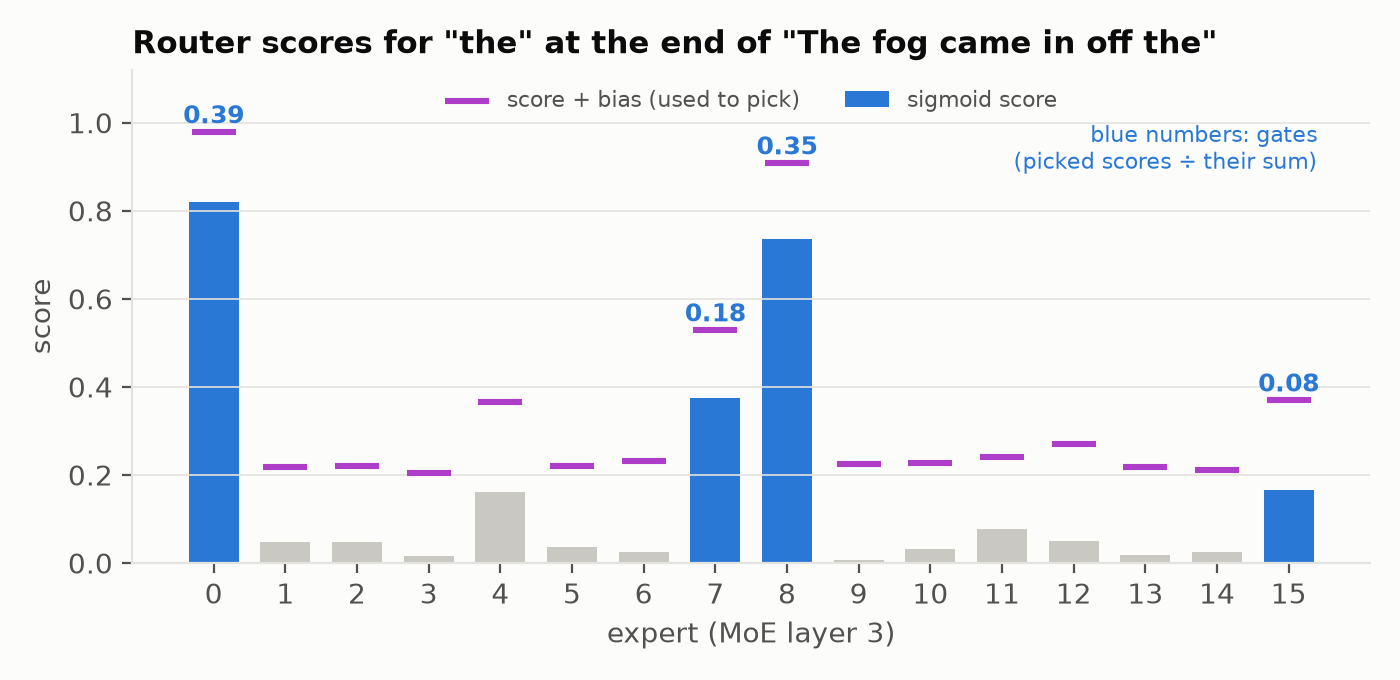
Usual FFN is a single big network that every token goes through whereas MoE replaces it with many small expert networks + a router. The router looks at each token as well as scores 16 experts and routes it to the top k, 4 in this case and the token's o/p is a weighted mix of those 4. On top of that 1 shared expert sees every token and handles the common stuff so the routed experts can work on specialization.
def swiglu(p, x):
    return (jax.nn.silu(x @ p["w1"]) * (x @ p["w3"])) @ p["w2"]            # [.., d] -> [.., h] -> [.., d]


def route(w_router, bias, x, cfg):
    scores = jax.nn.sigmoid(x.astype(jnp.float32) @ w_router.astype(jnp.float32))   # [N,E] affinity, in f32
    _, idx = jax.lax.top_k(scores + jax.lax.stop_gradient(bias), cfg.top_k)   # bias decides WHO is picked...
    picked = jax.nn.one_hot(idx, cfg.n_routed).sum(-2) > 0              # [N,E]
    gated = jnp.where(picked, scores, 0.0)                              # ...but gate values use raw scores
    return (gated / gated.sum(-1, keepdims=True) * cfg.route_scale).astype(x.dtype), scores


def moe(p, bias, x, cfg):
    B, T, d = x.shape
    xf = x.reshape(B * T, d)
    gates, scores = route(p["router"], bias, xf, cfg)                   # [N,E], [N,E]
    w = p["experts"]   # every expert runs on every token; unpicked experts get gate 0 (see post)
    h = jax.nn.silu(jnp.einsum("nd,edh->neh", xf, w["w1"])) * jnp.einsum("nd,edh->neh", xf, w["w3"])
    routed = jnp.einsum("ne,ned->nd", gates, jnp.einsum("neh,ehd->ned", h, w["w2"]))   # [N,d]
    out = routed + swiglu(p["shared"], xf)
    load = (gates > 0).mean(0) / cfg.top_k                              # [E] share of routed slots
    seq = seq_balance_loss(scores.reshape(B, T, -1), (gates > 0).reshape(B, T, -1), cfg)
    return out.reshape(B, T, d), {"load": load, "seq_loss": seq}
Balancing
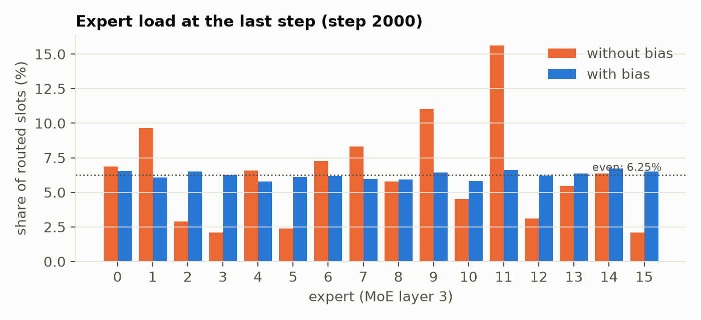
As mentioned previously, a router gets rather lazy when left alone for sometime. It might happen that a few experts must've been scoring well early so naturally more tokens will get routed to them and they would score even higher and then more tokens to them and so on which leads the others to starve. Usual fix is to add an auxiliary loss that would punish uneven routing but that can hurt the next word prediction quality.
V3 has no loss term instead adds a bias number to each expert where after every training step overloaded experts get their bias tuned down by 0.001, the underloaded ones gets an up + a backup loss that stops a single sequence from piling onto some of the experts.
def seq_balance_loss(scores, picked, cfg):
    # DeepSeek's tiny complementary loss: discourage any single sequence from piling onto few experts
    E, K, T = cfg.n_routed, cfg.top_k, scores.shape[1]
    f = picked.sum(1) * E / (K * T)                                     # [B,E] load, 1.0 = perfectly even
    P = (scores / scores.sum(-1, keepdims=True)).mean(1)                # [B,E] mean normalized affinity
    return cfg.alpha_seq * (f * P).sum(-1).mean()


def update_bias(biases, loads, gamma):
    # aux-loss-free balancing: after each step, nudge overloaded experts down and underloaded ones up
    return biases + gamma * jnp.sign(loads.mean(-1, keepdims=True) - loads)
Loss + MTP
Understanding loss is pretty simple -> if the unseen word gets high probability then the loss is less and vice versa. We train the model in manner that it adjusts the weights to make the loss smaller.
The usual model only learns to predict the next token whereas V3 adds a small module that enables the model to even guess the token after that which helps the model to plan a little ahead. It works like:
- take the model's final hidden state at position
iwhich already knows up to tokeni - take the embedding of the actual next token which is
i+1 - normalize both of them, put them together and then squash 768 (384*2) back to 384
- run that through a single dense transformer block
- and then use the same head as the main model to predict the next token
i+2
Hence the total loss becomes:
loss = main + .3 * mtp + tiny sequence balance loss (we discussed earlier)
def cross_entropy(logits, targets):
    logp = jax.nn.log_softmax(logits.astype(jnp.float32), -1)
    return -jnp.take_along_axis(logp, targets[..., None], -1).mean()


def loss_fn(params, biases, tokens, cfg):
    # tokens: [B, T + 1 + n_mtp]. Main model predicts t+1; MTP module k predicts t+1+k.
    T = tokens.shape[1] - 1 - cfg.n_mtp
    logits, h, aux, _ = forward(params, biases, tokens[:, :T], cfg)
    main = cross_entropy(logits, tokens[:, 1:T + 1])
    cos, sin = rope(cfg, jnp.arange(T))
    mtp = 0.0
    for k, m in enumerate(params["mtp"], start=1):
        # combine depth k-1's hidden state at i with the embedding of token i+k, then one more block
        e = params["embed"][tokens[:, k:T + k]]                           # shared embedding
        h = jnp.concatenate([rms_norm(h, m["norm_h"]), rms_norm(e, m["norm_e"])], -1) @ m["proj"]   # [B,T,d]
        h, _, _ = block(m["block"], None, h, cos, sin, cfg)
        mtp += cross_entropy(rms_norm(h, params["norm_f"]) @ params["head"], tokens[:, k + 1:T + k + 1])  # shared head
    mtp = mtp / cfg.n_mtp
    loss = main + cfg.mtp_lambda * mtp + aux["seq_loss"]
    return loss, {"loss": loss, "main": main, "mtp": mtp, "seq": aux["seq_loss"], "load": aux["load"]}
Training
Finally we are training!!! I'll just go through a single training step and you can imagine that for 12,000 times
- A single batch contains 32 chunks of 256 tokens
- The model runs and we get the loss
- Use
jax.value_and_gradto see through how each weight should change so that loss can be minimized - update the weights with AdamW optimizer
- and finally update the expert biases for load balancing
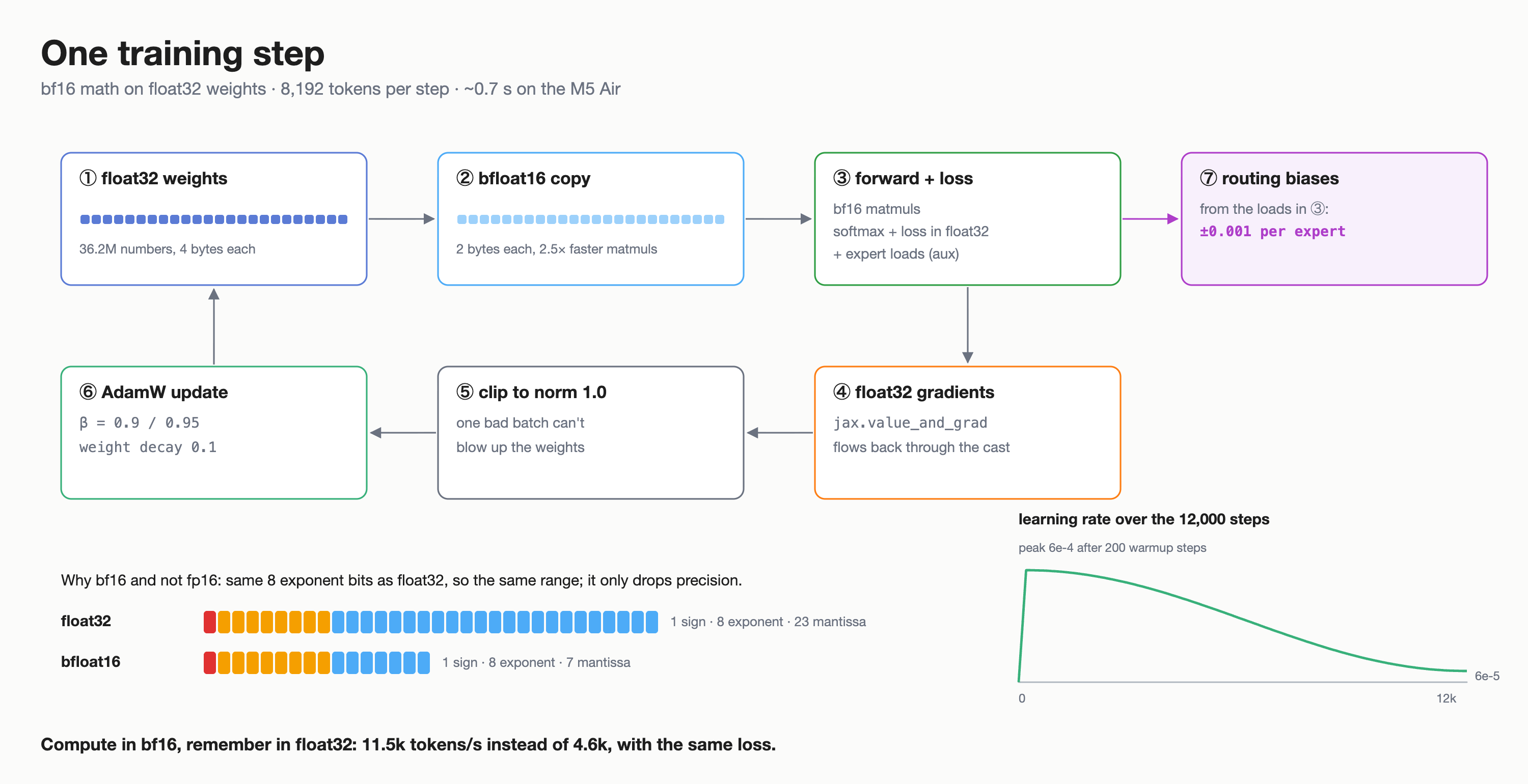
And as explained nicely in the other blogs (Saurabh's and Alessio's), @jax.jit decorator makes the whole step compiled once into a single XLA program and then that's reused for every step. Plus there's no .backward() in JAX, the gradient is just a function you call.
Coming to using bf16 which i talked about much earlier: the weights are stored as float32 but cast to bf16 for forward and backward passes so the matmuls run at bf16 speed instead and the small updates are still added in float32
def make_train_step(cfg, optimizer):
    cast = lambda p: jax.tree.map(lambda a: a.astype(cfg.dtype), p)      # mixed precision: f32 master weights

    @jax.jit
    def train_step(params, opt_state, biases, batch):
        loss = lambda p: loss_fn(cast(p), biases, batch, cfg)
        (_, metrics), grads = jax.value_and_grad(loss, has_aux=True)(params)
        updates, opt_state = optimizer.update(grads, opt_state, params)
        params = optax.apply_updates(params, updates)
        return params, opt_state, update_bias(biases, metrics["load"], cfg.gamma), metrics
    return train_step
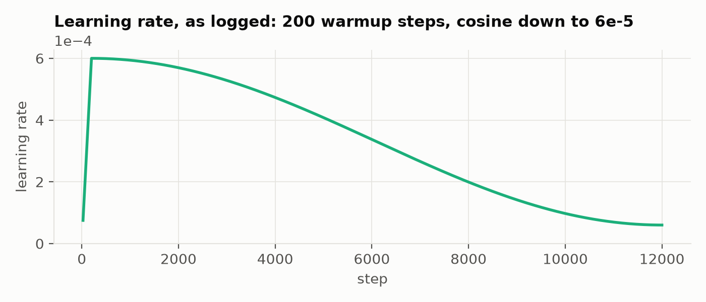
# train.py: AdamW with gradient clipping, 200 warmup steps, cosine decay to 6e-5
sched = optax.warmup_cosine_decay_schedule(0.0, 6e-4, 200, 12000, 6e-5)
opt = optax.chain(optax.clip_by_global_norm(1.0), optax.adamw(sched, b1=0.9, b2=0.95, weight_decay=0.1))
Generation and sampling
So now the model only does one thing: you give it some tokens and it scores every possible next token. Within that step is Prefill: which runs the complete prompt at once which fills the MLA cache with c and kr(the shared RoPE key) for every prompt token and Decode: which feeds in only the newest token and reuses the cache for everything before it and repeats. This covers how the generation happens.
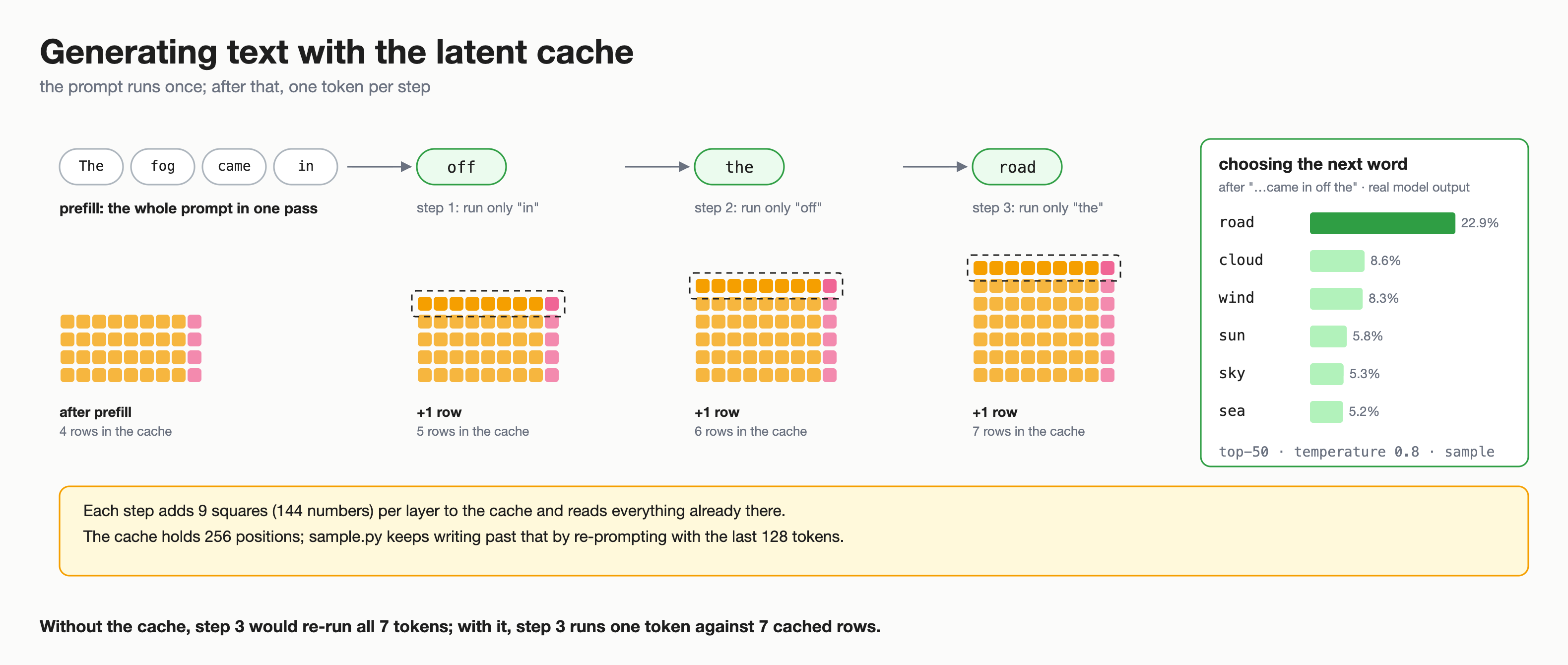
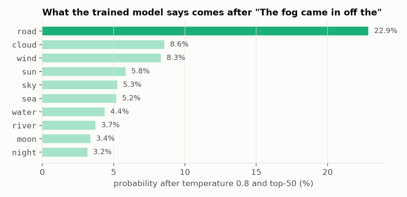
Coming to sampling: we are taking temperature=0.8with top-k 50 best tokens and picking randomly among them.
_forward = jax.jit(forward, static_argnames="cfg")

def sample_token(logits, key, temperature, top_k):
    if temperature == 0:
        return logits.argmax(-1)
    kth = jax.lax.top_k(logits, top_k)[0][:, -1:]                      # keep only the top_k logits
    return jax.random.categorical(key, jnp.where(logits < kth, -jnp.inf, logits) / temperature)

def generate(params, biases, prompt, n_new, cfg, key, temperature=0.8, top_k=50):
    B, P = prompt.shape
    if P + n_new > cfg.seq_len:
        raise ValueError(f"prompt ({P}) + new tokens ({n_new}) exceeds seq_len ({cfg.seq_len})")
    logits, _, _, caches = _forward(params, biases, prompt, cfg, init_cache(cfg, B, cfg.n_layers), 0)   # prefill
    out = [prompt]
    for i in range(n_new):                                              # then one token at a time
        key, sub = jax.random.split(key)
        out.append(sample_token(logits[:, -1], sub, temperature, top_k)[:, None])
        if i < n_new - 1:
            logits, _, _, caches = _forward(params, biases, out[-1], cfg, caches, P + i)
    return jnp.concatenate(out, 1)
Results
So finally we made it to results!!!
| Data | 207 books, 21.7M training tokens (Hammett repeated 3×); val is held-out crime fiction |
| Training | 12,000 steps, ~98M tokens (~4.5 epochs), ~2.6 h |
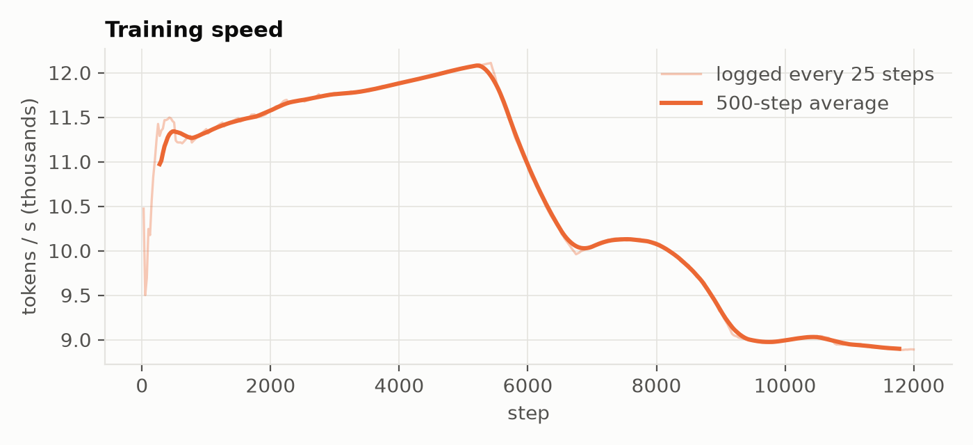
| Speed | ~10.7k tokens/s (median) |
| Val loss | 5.02 (step 250) → 3.51 |
| Train loss | 2.81 |
| MTP val loss | 3.68 |
| Expert load, with bias | 5.7–6.9% per expert, even is 6.25% (step 2000) |
| Expert load, without bias | 0.09–18.6% per expert (step 2000) |
| MLA cache | 144 numbers per token per layer, vs 480 for normal attention |
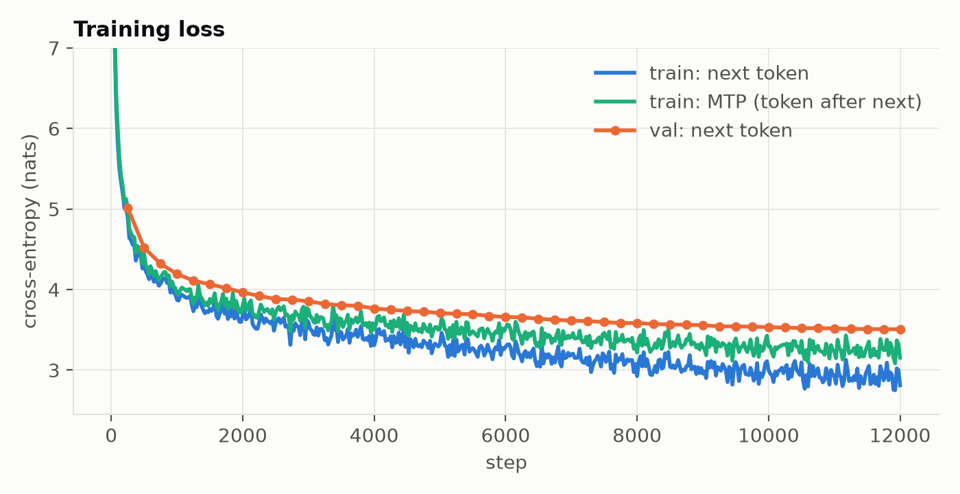
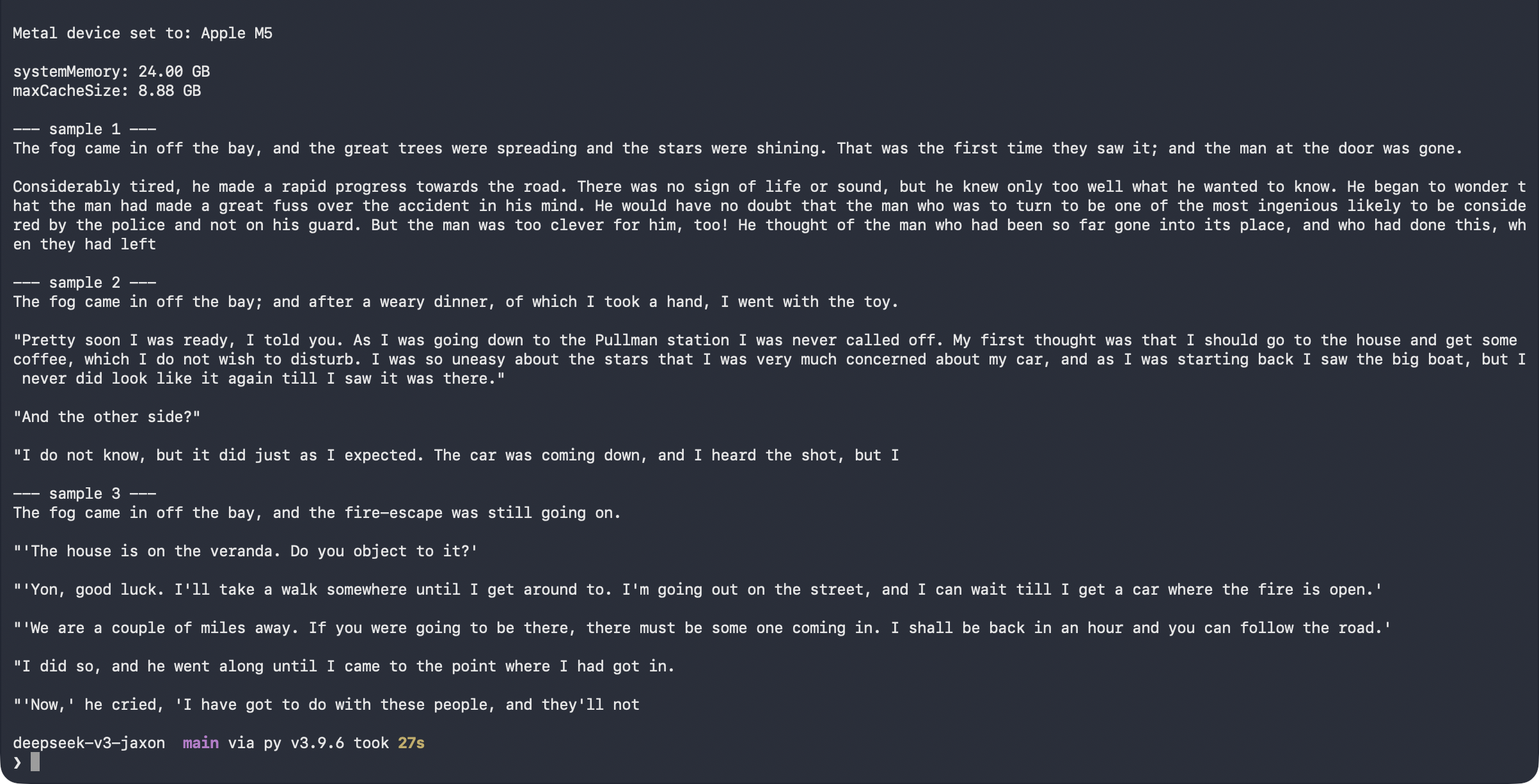
I believe i need more data than more steps to make it even better as its starting to memorize also it writes like a detective fiction sorta manner but ofcourse the story wouldn't hold together + the experts went from 0.09–18.6% to 5.7–6.9% and loss barely moved which really was DeepSeek's point.
Would love to have more feedback on what i could do better here as well as if i did anything wrong (X / email)! Most prolly i'll be moving to inference or mech interp now and exploring those!
Thanks for making it this far, hope you liked what you read :)